

When Should A Team Park the Bus?
/A model for optimizing intra-match tactical changes
Editor's note: This is the long version of this post. If you don't have 20 minutes to kill, then hop over to this abridged version.
By Jared Young (@jaredEyoung)
"Tottenham might as well have put the team bus in front of their goal," said Jose Mourinho in 2004 following a draw between his Chelsea club and the Spurs. Although he would later say the phrase was one typically used in Portugal, Mourinho was credited with coining the phrase 'parking the bus,' which described a team that was sitting the whole team behind the ball in an effort to block the goal. It's less frequent for team to play a full 90 minutes that way, but often teams with a lead will change tactics late in the game and park the bus in an effort to ensure victory. To do this they move their line of defensive pressure back toward the goal, committing more players to defense. The other team is allowed more possession of the ball but the bet is they'll have a lower chance of actually scoring the equalizer.
During this year’s FA Cup Final, Arsenal took a 1-0 lead over Aston Villa into halftime. They had thoroughly dominated the game and had taken eight shots to Aston Villa’s one. In that case, conventional wisdom was to change nothing at all. Arsenal logically kept up the pressure just as they did in the first half, added three more goals and finished with a shot advantage of sixteen to two.
The FA Cup Final shows us that it’s not always clear that a team should park the bus if they have a lead. Arsenal was in top form at that time, and were clearly the dominant side. They didn’t need to sit back defensively to ensure victory.
What are the factors that would indicate a team should change tactics, such as parking the bus? The goal of this post is walk through the building of a model that can be used to show teams when to park the bus and when to stay the course. The model will also be able to analyze other tactical choices.
What changes in a game when a team moves their pressure line back toward their goal? From a results point of view there are four key changes to consider. The first is that team down a goal will very likely increase the rate at which they shoot the ball. By lowering the pressure line, teams will concede possession and allow the opposition closer to the goal. This will result in more shots. The second change is that the team down a goal will finish a lower percentage of those shots. The point of committing more players to defense is to make it more difficult for the shooters to actually score - evidence of this trade-off to follow.
The third change is that the defensive team will shoot less often than they were previously. Conceding possession will mean they have the ball less and will have fewer chance to score. However, the fourth change is that the defensive team should be able to finish a higher percentage of their shots. This is the standard risk reward trade off of the counter attacking team. By sitting the defense deeper, they open up more space to cover when they get the ball. The best approach is to attack that space quickly, and when they do, they find fewer defenders to deal with and shoot at a higher percentage.
Here are charts that indicate that these four variables do move in relation to each other. The below chart shows that lowering the defensive pressure line does increase the rate at which opponents take shots. Passes allowed per defensive action is a metric that indicates how much pressure a team is putting on the ball. A higher number of passes per action indicates a low amount of pressure. A lower number of passes indicates a higher amount of pressure. This chart reveals that as defensive pressure is relaxed the opponent is able to take more shots.

The next chart shows that when one team takes more shots, the opposing team on average takes less shots. The blue points show the away shots are on the vertical axis and the home team is on the horizontal axis. If a home team takes twenty shots the blue line indicates that the away team will take on average about 10 shots. If an away team takes 20 shots a home team would take on average about 13. This graph reveals that a team’s shot taking frequency is indirectly related the rate of their opponent’s shots.

The next chart shows that as frequency of shots increases the finishing rate decreases. This aligns with what is expected; lower defensive pressure allows more shots but at a lower rate of success. As one team increases their shot taking frequency their finishing rate decreases and their opponents shot frequency while decrease while their finishing rate increases.

As an additional note, we can extract from the regression equation that the optimal number of shots to maximize goals scored is about 18 (18.1, in fact, using that old Calc I). Below is the resulting curve. This chart highlights why sitting deep can work if the opponents shot frequency is high enough. Expected goals scored actually goes down after teams shoot more than 18.1 shots per 90.

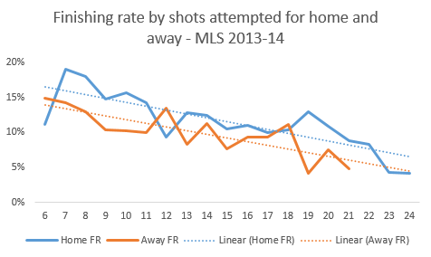
Since the relationship of two opposing teams' shot frequency differs between home and away teams, the finishing rate model needs to separate the two instances. Here is a chart of the MLS finishing rates by shots attempted split by home and away. There is about a 1.5% difference in finishing rates between home and away team, and this difference is even across all shot frequencies.
Changing the four variables for home and away teams - opponent shots, opponent finishing rate, team shots, team finishing rate - is the basis of this tactical model to determine the impact of changing the defensive pressure line. Before the model is built there needs to be some simplifying assumptions. Later in the post, more data will be analyzed that will allow some of these assumptions to be relaxed, resulting in a more accurate model.
The five key assumptions:
1. Shots occur in a uniform distribution. Example: If a team is going to take three shots in a ten minute period this assumption means that those shots would happen randomly across the ten minutes, and there would be no bias to them happening earlier or later in the ten minute period.
2. The teams in the model represent average teams. There will be teams, as in the Arsenal versus Aston Villa example, where one team is clearly dominant over another. This model will initially only look at these curves as an average.
3. Finishing Rate does not change as the game goes on. We will examine this assumption later on as it does appear that in certain situations, finishing rate increases as the game matures, but for now, let’s keep this simple.
4. The team setting the defensive pressure line is still looking to score. This basically means that a team that is focusing on defense will still try to score on the counter and won’t just kick the ball back to the offense once they gain possession. This is important because it means that a coach’s objective is more than just stopping a goal, it is to increase the team’s chance of scoring the next goal. This will be the objective of the model.
5. The game state will not impact finishing rates based on shots taken. This assumption will say that the impact of shot frequency on finishing rate will not change as the score changes. For example, the finishing rate will be the same if the score is 1-0 or 0-0. As the model specifically looks at parking the bus this assumption will need to be challenged.
The model
Combining these curves and assumptions together the model can now be built to determine the impact of changing the tactic in question. Here's and example of how the model will work – an away team is up one in the 80th minute, and they reduce their pressure line so that the home team is now shooting at a rate of 25 shots per 90. The away team would now only be shooting at a rate of 8.5 shots per game. With just 10 minutes to go, the away team is forecasted to average under 2 shots while the home team is going to shoot nearly 6. The home team will have a finishing rate of about 5% and the away team, now striking on the counter, will have a finishing rate of 14%. Is that a good move? The answer of course is, it depends.
Example one: Away team up one goal
Here is the first model output chart to examine. The blue and orange points in these charts reveal the shots attempted in relation to each other. The gray line in this case represents the probability that the away team will score the next goal.

Given the gray curve is U-shaped the best tactical move is going to be a function of where a team currently sits on the curve. Let’s take an example where the away team is up one goal and both teams are attempting shots at the exact same rate, at 12.2 shots per 90. This would be where the orange and blue lines intersect. The away team has a 47% chance of scoring the next goal because away teams have a lower finishing rate than home teams, all other factors equal. Of course the away coach wants to make a tactical change to increase those chances, and there are two options. The team can attempt to possess the ball more and create more shots. If they can increase their shots to 14 per 90 then they increase the likelihood of scoring the next goal to 60%. They could also choose to bunker in and reduce their possession. However, in order to improve their chances of scoring the next goal they would need to allow the home team to shoot the ball at about 30 shots per 90 minutes, or once every 3 minutes. That means they would have to sit very deep to allow that to happen. The change would be extreme. It would be less of a change and possibly make more sense to attempt increase possession.
The team could attempt to push for more possession and if they see the game going in the wrong direction, they could then opt to sit deep. However, the model shows that in order for parking the bus to make sense, a team must fully commit. Going part of the way appears to be very dangerous as the odds of scoring the next goal can decrease to as low as 40%.
Example two: Home team up one goal
Now the home team is up one goal in the 80th minute. They will take more shots relative to away team shots and will finish them at a higher rate as well. The result of those two improvements is shown in the following chart.

There is far more upside for the home team to bunker down and secure the win due to the fact that the away team will be expected to get off fewer shots and finish less of them. The home team will always have at least a 50% chance of scoring the next goal, but they can give themselves up to a 90% chance by sitting deeper on defense.
Again it becomes clear that where a team sits on the gray curve during the course of a game should give the coach the best indication of when and in which direction the team should try to move.
Going back to the Arsenal - Aston Villa FA Cup Final example
Given Arsenal’s dominance in the game assume Arsenal had a home team advantage. At half time they have eight shots, or a rate of sixteen per 90 minutes. The away team should be shooting six shots per 90, but at halftime had only mustered one attempt. Given Arsenal’s shooting frequency rate of sixteen the model says they have a 70% chance of scoring the next goal. Given Aston Villa wasn’t even shooting at their expected shooting frequency, the odds were much much greater. In order to improve their chances of scoring the next goal Arsene Wenger would have had to employ an extremely bunkered defense to increase their odds. It clearly made little sense to make such a shift and this model highlights the math behind that decision.
Relaxing the earlier assumptions
While this model gives a good sense of the trade-off between gaining possession and playing bunker and counter soccer, there are opportunities to make some of the assumptions more realistic. The most challenging to adjust for are the first two assumptions The first, the uniform distribution of shot frequency is difficult to challenge because at this point the model is only assuming what style of play a team is playing, based on the rate at which the average team allows and takes shots. To understand the frequency of shot taking and whether or not they accelerate or decelerate over time the model would need to understand exactly what is happening over the period of time being analyzed. Much better data would be needed to analyze this phenomenon in more detail.
2. The teams in the model represent average teams. The average curves could be adjusted for specific teams or groups of teams. That could be the subject of future study on the model, but the issue would be getting enough shots to build curves with statistical significance. This model already uses two full seasons of an entire league’s worth of data, and while trends are clear, there is a fair amount of variation in the subsegments.
3. Finishing Rate does not change as the game goes on. This one is easy enough to examine, but also not easy to adjust for, as will be clear after looking at the following charts.
Here is a chart of finishing rate over time in MLS in 2013 and 2014.

There is a pretty strong upward trend when looking at finishing rate by time. It’s maybe not as dramatic as the best fit line reveals. The first ten minutes of a game have the lowest finishing rates by far. Between minute 11 and minute 70 there is a big increase but the line is reasonably flat, or at least there is no discernable trend. Then there is another step change after minute 70 that lasts through the rest of the game. Should this be a factor in the model? It at first glance certainly appears so. But there could be other factors, beyond time that are driving the change.
Here is a chart of finishing rates by time when the home team is up one goal.

The finishing rate for the home team explodes after the 90th minute. This is no doubt influenced by the home team getting counter attacking chances as the away team brings more bodies forward to try to equalize. You can see too that the away team’s finishing rate goes down after the 90th minute. However, between the 11th minute and the 90th minute the home team’s finishing rate is relatively flat, with a slight gradual increase. The away team’s trend is flat.
Here is a chart of the finishing rates over time if the away team is up one goal.

With the away team up a goal, both teams actually finish a slightly lower rate of shots as the game progresses.
It appears as though the need to adjust the model by time of game is not as important as the first graph indicated. The increase in finishing rate in total appears to be more of a function of game state and adjusting tactics than simply the game maturing. There’s probably some nuance to add to the model here but at this state, the assumption will stay flat.
The fourth assumption, the team setting the defensive pressure line is still looking to score is more a formality as it’s rather obvious that a team should try to score when given the chance. The assumption was more to gain alignment on the objective of the model which is to increase the likelihood to score the next goal. In some cases a coach could be looking to minimize the likelihood that the team allows two goals, but that could be the subject of another post.
Trying to score a goal despite being up one does have some value but not as much as one would think. This model plus the use of the binomial distribution, to calculate the probability of different goal outcomes, can help calculate that value of trying to score. For example if an away team, up one goal, does not try to score from the 70th minute on and they are allowing shots at a frequency of 20 shots per 90 then they should expect to earn 2.21 points in that game. Adding in the away team’s potential to score one or more goals in the next 20 minutes, their expected points per game increases to 2.29. More, but not a ton more.
The last assumption is where the model can be stretched with the data available. The last assumption states that game state will not influence finishing rate as a function of shots attempted per 90. We’ve already seen that game state does indeed influence finishing rates so we just need to adjust them for shots attempted.
Relaxing the game state assumption – Away team up one goal
Starting with the scenario where the away team is up one goal here are charts of how the actuals play out against the originally modeled curves. The expected curve is what was used in the model prior. The actual curves will be considered in the game state adjusted model.

The first chart shows that the home team will get increasingly more shots as the game matures relative the away team’s shot frequency. Essentially an away team coach who is nursing the lead should understand that the home team will be shooting increasingly more relative to how his team is shooting.

Compounding the issue is the fact that away teams, when up a goal, get shots off less frequently than average relative to the frequency of home shots. Defensive pressure line being normalized, away teams just don’t shoot as frequently when in the lead.

When down a goal, the home team finishes as expected given the rate at which they are shooting.

Not only do away teams shoot less frequently than expected when up a goal, but their finishing rate is consistently lower as well.
Taking these factors into account the model is adjusted as follows:

The gray line represents the original model curve. The yellow curve now represents the odds adjusted for game state at half time. In the case of the away team being up one, they end up shooting less frequently and finishing a lower percentage of those shots than the unadjusted model suggests, so in reality, they have a much lower likelihood of scoring the next goal. Notice the model actually shifts slightly in favor of possessing the ball. The yellow and gray lines converge just a bit as the away team takes more shots.
However, when factoring the evidence that suggests the home team will attempt relatively more shots as the game progresses (the first chart in this section), that factor disappears as the game wears on. The dark blue line shows what the curve looks like in the 70th minute. As the game evolves the park the bus strategy gets more and more appealing. Somewhere between halftime and the 70th minute it makes more sense to employ an extremely low defensive line than it does to try to maintain an extreme level possession.
Relaxing the game state assumption – Home team up one goal
Here are the four charts for the scenario where the home team is up a goal. The game state impacts are similar but less pronounced for the home team.

Just like the home team in the away team up one goal scenario, the away team down a goal increasingly earns shots that are not expected given the opposition’s shot frequency. The increase is not as pronounced as the other scenario but will have a similar impact.

Home teams shoot less frequently with a lead relative to away shot frequency.

Away shots converge to the expected level as the game progresses, but there is a fairly wide gap for most of the game. Perhaps away team’s try too hard early on for the equalizer.

The home team finishing rate is suppressed slightly for most of the game, except for that explosion in injury time.
Overall the game state impacts are similar in both the away team up one and the home team up one scenarios. In the case of the home team being up one goal the impacts are muted, which will improve the chances of the home team relative to how game state impacted the away teams.

Without game state adjustments, the home team gained much more from sitter deeper than the away team. That state continues despite the flattening of the curve over time. As the game goes on it appears like this advantage weakens. The dark blue curve shows a flattening of the tactical options as the game matures.
Closing thoughts
First of all, if you made it this far, I very much appreciate you taking the time to soak this in. There are a couple of key points I believe this model brings to light that I want to highlight.
1. A team should push for either extreme possession or extreme concession. Playing in the middle, in any game state, reduces a team’s chances of scoring the next goal. Coaches should commit to one pressure line tactic or the other and not remain in no man’s land. This seems at odds with how a number of MLS teams operate.
2. Which approach the coach chooses should be a function of where on the curve the game is currently being played. In the case of the Arsenal versus Aston Villa FA Cup Final, it made sense for Arsene Wenger to maintain their position of control. If an away or home team is up one and is losing the shots against battle, sitting deeper will be a more effective tactic to increase their odds of scoring the next goal.
3. Counter to current thinking, a home team with a goal advantage stands to improve their odds of winning more by parking the bus than an away team in the same situation. Current thinking, I believe, says the away team should bunker in to get the three points and the home team should try to control possession. This model contradicts that logic because the home team will be finishing a higher rate of shots at home and will produce more shots than expected, making a counter strategy more appealing.
4. The limits on the model can be stretched further to address the following questions:
a. Does the effectiveness of a low defensive line diminish over time? Are the odds of success consistent over 30 minutes or does the tactic have a limited shelf life?
b. How do the curves change when a good team is playing against a poor team?
c. Can data be collected by Opta or another provider to better understand the impact of defensive pressure lines on shots attempted?
And I’m sure there are many other questions and ways to push the model. Please let me know if you have any at @Jaredeyoung on twitter. Next time your team is up a goal and looking to finish off a game, how do they approach it?