

Predicting Goals Scored using the Binomial Distribution
/Much is made of the use of the Poisson distribution to predict game outcomes in soccer. Much less attention is paid to the use of the binomial distribution. The reason is a matter of convenience. To predict goals using a Poisson distribution, “all” that is needed is the expected goals scored (lambda). To use the binomial distribution, you would need to both know the number of shots taken (n) and the rate at which those shots are turned into goals (p). But if you have sufficient data, it may be a better way to analyze certain tactical decisions in a match. First, let’s examine if the binomial distribution is actually dependable as a model framework. Here is the chart that shows how frequently a certain number of shots were taken in a MLS match.
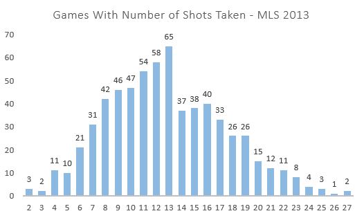
The chart resembles a binomial distribution with right skew with the exception of the big bite taken out of the chart starting with 14 shots. How many shots are taken in a game is a function of many things, not the least of which are tactical decisions made by the club. For example it would be difficult to take 27 shots unless the opposing team were sitting back and defending and not looking to possess the ball. Deliberate counterattacking strategies may very well result in few shots taken but the strategy is supposed to provide chances in a more open field.
Out of curiosity let’s look at the average shot location by shots taken to see if there are any clues about the influence of tactics. To estimate this I looked expected goals by each shot total. This does not have any direct influence on the binomial analysis but could come in useful when we look for applications.

The average MLS finishing rate was just over 10 percent in 2013. You can see that, at more than 10 shots per game, the expected finishing rate stays constant right at that 10-percent rate. This indicates that above 10 shots, the location distribution of those shots is typical of MLS games. However, at fewer than 10 shots you can see that the expected goal scoring rate dips consistently below 10%. This indicates that teams that take fewer shots in a game also take those shots from worse locations on average.
The next element in the binomial distribution is the actual finishing rate by number of shots taken.

Here it’s plain that the number of shots taken has a dramatic impact on the accuracy rate of each shot. This speaks to the tactics and pace of play involved in taking different shot amounts. A team able to squeeze off more than 20 shots is likely facing a packed box and a defense less interested in ball possession. What’s fascinating then is that teams that take few shots in a game have a significantly higher rate of success despite the fact that they are taking shots from farther out. This indicates that those teams are taking shots with significantly less pressure. This could indicate shots taken during a counterattack where the field of play is more wide open.
Combining the finishing accuracy model curve with number of shots we can project expected goals per game based on number of shots taken.

What’s interesting here is that the expected number of goals scored plateaus at about 18 shots and begins to decline after 23 shots. This, of course, must be a function of the intensity of the defense they are facing for those shots because we know their shot location is not significantly different. This model is the basis by which I will simulate tactical decisions throughout a game in Part II of this post.
Now we have the two key pieces to see if the binomial distribution is a good predictor of goals scored using total shots taken and finishing rate by number of shots taken. As a refresher, since most of us haven’t taken a stat class in a while, the probability mass function of the binomial distribution looks like the following:

Where:
n is the number of shots
p is the probability of success in each shot
k is the number of successful shots
Below I compare the actual distribution to the binomial distribution using 13 shots (since 13 is the mode number of shots from 2013’s data set), assuming a 10.05% finishing rate.

The binomial distribution under predicts scoring 2 goals and over predicts all other options. Overall the expected goals are close (1.369 actual to 1.362 binomial). The Poisson is similar to the binomial but the average error of the binomial is 12% better than the Poisson.
If we take the average of these distributions between 8 and 13 shots (where the sample size is greater than 40) the bumps smooth out.

The binomial distribution seems to do well to project the actual number of goals scored in a game, and the average binomial error is 23% lower than with the Poisson. When individually looking at shots taken 7 to 16 the binomial has 19% lower error if we just observe goal outcomes 0 and 1. But so what? Isn’t it near impossible to predict the number of shots a team will take in the game? It is. But there may be tactical decisions like counterattacking where we can look at shots taken and determine if the strategy was correct or not. And a model where the final stage of estimation is governed by the binomial distribution appears to be a compelling model for that analysis. In part II I will explore some possible applications of the model.
Jared Young writes for Brotherly Game, SB Nation's Philadelphia Union blog. This is his first post for American Soccer Analysis, and we're excited to have him!